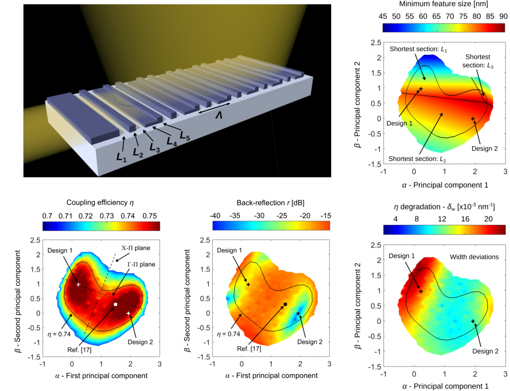
In this paper we tackle a problem that is frequent to many disciplines and is getting more and more common also in photonics: the need to handle simultaneously many parameters when we design a device or a component. We do so by making use of machine learning dimensionality reduction. By developing this design method we also show another interesting thing. Using machine learning does not necessarily means giving up all our previous knowledge about the physics of photonic devices to let the machine “do our job”. Quite the contrary!
Machine-learning algorithms can be a powerful addition in our toolbox to handle problems that would be difficult to solve with more traditional approaches.
A bit of background. When we have to create, study, and design a new device in photonics we commonly proceed relying on our theoretical knowledge and intuition to identify the potential structure and design parameters range. We then explore the parameter space combining analytical and numerical tools. We fix some of the parameters to reasonable values, we sweep the remaining ones, simulate the device response, and iterate until we have a good understanding of the general behavior and the effect that each parameter has on it. This approach gives the designer a great insight on how a device works but it has also limitations. It assumes the evaluation process can be decomposed into sequential steps and the amount of computational resources that are normally required constrains its scope to structures governed by only few parameters.
As complexity of photonics grows (think for example to metamaterials) this classical approach poses increasing challenges. Intuitively, having more “knobs” (parameters) to play with gives us more possibilities to design devices with complex behaviors but also makes it more difficult to do so. It is not just about numbers. Parameters are often strongly inter-dependent and optimizing them sequentially is no longer applicable. Clearly also a brute-force exhaustive exploration of all the possible parameter combinations is not possible as it would require hundreds of years of simulations! This is the reason why optimization algorithms (e.g. genetic optimization or particle swarm) became so popular in the field in the last few years. They can efficiently handle many parameters and yield high-performance design with a reasonable computational effort (mainly in terms of the total time the algorithm takes to converge to an acceptable solution, i.e. often the total number of simulations it requires). Performance in this context can be anything, a metric we use to evaluate the behavior of our device. More recently also supervised machine learning methods such as the artificial neural network attracted a lot of interest. While all these approaches represent significant improvements to the design flow, they still have some constitutive limitations:
- usually a single performance criterion is optimized;
- only a single or a handful of optimized designs are discovered;
- the optimization process needs to be repeated from scratch if we discover down the road that different or additional performance criteria must be considered (this is a new device after all!).

Furthermore, once we obtained our optimized design it reveals very little on the characteristics of the design space and the influence of the design parameters on the device performance. It is essentially rather hard to understand the device behavior without further investigations. For all this reasons we decided to deal with this problem in a different way.
The fundamental trick here is to focus our attention only on that little part of the parameter space that actually brings to devices with high performance.
We do this by introducing a three-stage process. We start choosing a primary performance criterion that is of particular importance (e.g. losses of a power splitter or coupling efficiency of a grating coupler). Devices that do not provide high performance measured with this criterion are not of interest. In the first stage then we use an optimization algorithm to generate a sparse collection of different good designs, i.e. designs that optimize the primary criterion (Fig. a). Supervised machine learning techniques can be exploited to speed up the search process by quickly providing promising design candidates as starting points for the optimizer. In the second stage (Fig. b), dimensionality reduction is applied to analyze the relationship in the parameter space between these designs. The goal here is to find a smaller number of parameters that can still well describe all good designs we have found in the first stage. In the last stage (Fig. c) we can eventually proceed in a very classical way: we map the design sub-space by sweeping the new small set of parameters. We can do this not only for the primary performance criterion we have selected at the beginning but we can map any additional criteria with a limited computational effort.

The beauty of this approach is also that it does not necessarily require a lot of data to work properly. In the paper we demonstrate the design of a perfectly vertical grating coupler and we begin with a set of only five different designs with high fiber coupling efficiency!
Through this process, the sparse initial set of good designs efficiently leads to the identification and comprehensive characterization of the continuum of all good designs.
This highlights their performance as well as structural differences and limitations. Even if many parameters are involved, this approach allows the designer to obtain insights on the behavior of the device and a clear understanding of the design space, making possible the discovery of superior designs based on the relative priorities for a particular application.
If you want to learn more, all the details are in the paper and the supplementary material! Link: https://www.nature.com/articles/s41467-019-12698-1
